BBN reaction rates vs the Hubble rate

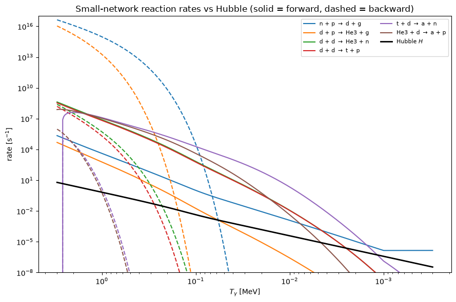
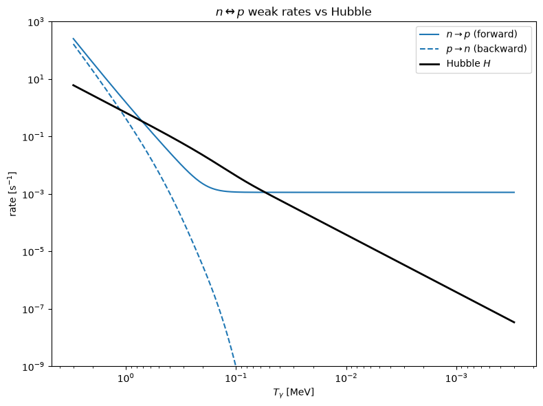
Plots the temperature dependence of the reaction rates that drive BBN, all expressed as inverse times \([\mathrm{s}^{-1}]\) so they can be compared directly with the cosmological expansion rate \(H(T)\) (black). A reaction is efficient while its rate exceeds \(H\) and freezes out once it drops below \(H\), so the crossings of each curve with the black line mark the key epochs of nucleosynthesis.

Two panels:

1. Weak rates \(n\leftrightarrow p\) (forward \(n\to p\) solid, backward \(p\to n\) dashed). These are already normalised inverse times; their crossing with \(H\) near \(T_\gamma\simeq0.8\) MeV sets the neutron-to-proton freeze-out ratio, and \(n\to p\) flattens at low \(T\) to the free-neutron decay rate \(1/\tau_n\).

2. Main nuclear reactions of the small network (forward solid, backward dashed, one colour per reaction). The forward rates sit far above \(H\) (the light network is in nuclear statistical equilibrium), while the backward photodissociation rates (e.g. \(d+\gamma\to n+p\)) dominate at high \(T\) and collapse as the plasma cools — the “deuterium bottleneck” that delays nucleosynthesis until \(T_\gamma\simeq0.07\) MeV.

See PRIMAT’s Physics Reports review (Pitrou, Coc, Uzan, Vangioni 2018) for the definitions of the reaction rates and the weak \(n\leftrightarrow p\) rates used here.

import importlib.util, subprocess, sys

# In Colab (or any environment without a local primat checkout), pip-install
# the released package; local dev runs already have it importable (editable
# install / repo on sys.path via the cell below), so this is a no-op there.
if importlib.util.find_spec("primat") is None:
    subprocess.run([sys.executable, "-m", "pip", "install", "-q", "primat"], check=True)

import sys, os
sys.path.insert(0, os.path.abspath('..'))

import numpy as np
import matplotlib.pyplot as plt
from primat.main import PRIMAT
from primat.network_data import reaction_stoichiometry, reaction_display_name

# A single small-network PRIMAT build gives us everything we need:
#   * run.background -- the cosmological background, exposing the Hubble rate
#     H(T) [s^-1], the baryon mass density rho_B(T) [g/cm^3], and the
#     already-normalised n<->p weak rates [s^-1];
#   * run.nucl._lt_net -- the compiled low-temperature nuclear network, whose
#     fill_buffer(T) returns the forward/backward reaction-rate coefficients
#     (the same ones the ODE right-hand side integrates).
# We only build the background + rate tables here; we never call solve(),
# because these rates are properties of the plasma temperature alone, not of
# a particular abundance history.
run = PRIMAT({'network': 'small'})
bg, nucl, cfg = run.background, run.nucl, run.cfg
lt = nucl._lt_net                      # low-T NetworkDefinition
print('Reactions in the small network:', lt.names)

Reactions in the small network: ['n__p', 'n_p__d_g', 'd_p__He3_g', 'd_d__He3_n', 'd_d__t_p', 't_p__a_g', 't_d__a_n', 't_a__Li7_g', 'He3_n__t_p', 'He3_d__a_p', 'He3_a__Be7_g', 'Be7_n__Li7_p', 'Li7_p__a_a']

# Photon-temperature grid, high -> low (MeV). The x-axis is inverted below so
# time flows left -> right (hot early Universe on the left).
T_MeV = np.logspace(np.log10(3.0), np.log10(3e-4), 400)
T_K = T_MeV * cfg.MeV_to_Kelvin


def hubble_of_T(T_MeV):
    """Friedmann expansion rate H(T_gamma) [s^-1] on the temperature grid.

    background.Hubble() needs the three flavour neutrino temperatures as well
    as T_gamma; we read them from the non-instantaneous-decoupling history at
    the cosmic time t(T_gamma) of each grid point (falling back to
    T_nu = T_gamma if no neutrino history is attached).
    """
    H = np.empty_like(T_MeV)
    for i, Tm in enumerate(T_MeV):
        t = float(bg.t_of_T(Tm))
        tnu = bg.Tnu_of_t(t)
        if tnu is None:
            H[i] = bg.Hubble(Tm, Tm, Tm, Tm)
        else:
            H[i] = bg.Hubble(Tm, tnu['e'], tnu['mu'], tnu['tau'])
    return H


# Baryon mass density rho_B(T) [g/cm^3] at each grid point. This is the
# prefactor that converts a nuclear rate *coefficient* into an inverse time
# (see reaction_rate below).
rho_B = np.array([bg.rhoB_BBN(float(bg.t_of_T(Tm))) for Tm in T_MeV])

# Fill the forward/backward rate buffer at every temperature. Layout (see
# NetworkDefinition.fill_buffer): r[0]/r[1] are the weak n->p / p->n rates,
# and for reaction k (>=1) r[2k]/r[2k+1] are its forward/backward coefficient.
# clamp=False keeps the raw detailed-balance reverse rate (no low-T cap), so
# the backward curves are the true physical rates rather than the solver's
# stability-clamped values.
buffers = np.array([
    lt.fill_buffer(tk, bg.weak_nTOp_frwrd, bg.weak_nTOp_bkwrd, clamp=False).copy()
    for tk in T_K])


def weak_rates():
    """(n->p, p->n) weak rates [s^-1] on the grid (already inverse times)."""
    return buffers[:, 0], buffers[:, 1]


def reaction_rate(name):
    """Forward and backward rate of reaction ``name`` as inverse times [s^-1].

    The nuclear network integrates dY_i/dt from fluxes
    F = coeff * rho_B**(n-1) * prod(Y), where n is the number of nuclei on
    that side of the reaction (see primat.network_builder). Because PRIMAT's
    abundances Y are dimensionless number fractions, the group
    ``coeff * rho_B**(n-1)`` already carries units of s^-1: it is exactly the
    reaction-rate coefficient the solver multiplies onto the abundance
    monomial, i.e. the rate per unit reactant fraction. That is what we plot,
    so the comparison with H(T) is apples-to-apples.

    The forward side uses R = number of reactants; the backward side uses
    P = number of products (photons are not counted — they are folded into
    the detailed-balance coefficient), matching the rho powers in the RHS.
    """
    k = lt.names.index(name)
    reactants, products = reaction_stoichiometry(name)
    R, P = sum(reactants.values()), sum(products.values())
    forward = buffers[:, 2 * k] * rho_B ** (R - 1)
    backward = buffers[:, 2 * k + 1] * rho_B ** (P - 1)
    return forward, backward


H = hubble_of_T(T_MeV)

Weak \(n\leftrightarrow p\) rates

The forward \(n\to p\) (solid) and backward \(p\to n\) (dashed) rates cross the Hubble line near \(T_\gamma\simeq0.8\) MeV: this is weak freeze-out, which fixes the neutron-to-proton ratio that seeds essentially all the \(^4\)He. Below \(\sim0.1\) MeV the \(n\to p\) curve flattens onto the constant free-neutron decay rate \(1/\tau_n\).

npr, pnr = weak_rates()

fig, ax = plt.subplots(figsize=(8, 6))
ax.loglog(T_MeV, npr, color='C0', ls='-',  label=r'$n\to p$ (forward)')
ax.loglog(T_MeV, pnr, color='C0', ls='--', label=r'$p\to n$ (backward)')
ax.loglog(T_MeV, H,   color='black', lw=2, label=r'Hubble $H$')
ax.invert_xaxis()                      # hot (early) on the left
ax.set_xlabel(r'$T_\gamma$ [MeV]')
ax.set_ylabel(r'rate [s$^{-1}$]')
# Span down to ~1e-9 so the low-T tail is visible: p->n falls far below H,
# while n->p flattens onto the constant free-neutron decay rate 1/tau_n.
ax.set_ylim(1e-9, 1e3)
ax.set_title(r'$n\leftrightarrow p$ weak rates vs Hubble')
ax.legend()
fig.tight_layout()
fig.savefig('plots/reaction_rates_weak.pdf', bbox_inches='tight')
plt.show()

Main nuclear reactions of the small network

Forward rates (solid) and their detailed-balance backward rates (dashed), one colour per reaction. The forward rates sit orders of magnitude above \(H\) — the light network is in nuclear statistical equilibrium once deuterium forms — while the backward photodissociation rates dominate at high \(T\) (abundant energetic photons) and fall steeply as the plasma cools. The delay of nucleosynthesis until the backward \(d+\gamma\to n+p\) rate drops below the forward \(n+p\to d+\gamma\) rate is the classic deuterium bottleneck.

Set reactions = lt.names[1:] to plot all 12 reactions instead of the curated main channels.

# Curated main channels of the small network (n+p->d and the leading
# deuterium-burning / mass-3 / mass-4 reactions). Swap for lt.names[1:] to
# show all 12 reactions.
reactions = ['n_p__d_g', 'd_p__He3_g', 'd_d__He3_n',
             'd_d__t_p', 't_d__a_n', 'He3_d__a_p']

fig, ax = plt.subplots(figsize=(9, 6))
for j, name in enumerate(reactions):
    forward, backward = reaction_rate(name)
    color = f'C{j}'
    label = reaction_display_name(name).replace(' > ', r' $\to$ ')
    ax.loglog(T_MeV, forward,  color=color, ls='-',  label=label)
    ax.loglog(T_MeV, backward, color=color, ls='--')          # backward: no label
ax.loglog(T_MeV, H, color='black', lw=2, label=r'Hubble $H$')
ax.invert_xaxis()
ax.set_xlabel(r'$T_\gamma$ [MeV]')
ax.set_ylabel(r'rate [s$^{-1}$]')
# Wide y-range: the backward photodissociation rates reach ~1e16 s^-1 when
# the plasma is hot, while H(T) falls to ~1e-6 s^-1 at the end of BBN, so
# span ~1e-8..1e17 to show every curve's full extent and its crossing with H.
ax.set_ylim(1e-8, 1e17)
ax.set_title('Small-network reaction rates vs Hubble '
             '(solid = forward, dashed = backward)')
ax.legend(fontsize=8, ncol=2)
fig.tight_layout()
fig.savefig('plots/reaction_rates_nuclear.pdf', bbox_inches='tight')
plt.show()