
Sensitivity of BBN observables to physical parameters
What this notebook computes
We compute the logarithmic sensitivity of each BBN observable \(O\) to each physical parameter \(p\): $\( S(O, p) \equiv \frac{\partial \ln O}{\partial \ln p} \approx \frac{\ln O(p\,(1+\delta)) - \ln O(p\,(1-\delta))}{2\,\ln(1 + \delta)}, \)\( evaluated by a symmetric finite difference with a 1% step (\)\delta = 0.01$).
This dimensionless number tells you: if parameter \(p\) changes by 1%, by what percentage does observable \(O\) change?
Since primat 1.x this is a one-call public API,
primat.sensitivity.sensitivity_table
(see the How-to → Sensitivity tables guide). This notebook is now a thin
demo of that API: it builds the list of parameters to vary, calls
sensitivity_table once, and plots the returned matrix. The heavy lifting
— running two bracketing BBN solves per parameter on the fast C backend and
sharing a single central solve — happens inside the API.
Parameters varied
Group |
Parameters |
Mechanism |
|---|---|---|
Nuclear rates |
All 12 key reaction rates |
|
Weak sector |
Neutron lifetime τ_n |
|
Gravity |
Newton constant G_N |
|
Cosmology |
Baryon density Ω_b h², ΔNeff |
|
Observables
\(Y_P\) (He-4 mass fraction), D/H, ³He/H, ⁷Li/H
import importlib.util, subprocess, sys

# In Colab (or any environment without a local primat checkout), pip-install
# the released package; local dev runs already have it importable (editable
# install / repo on sys.path via the cell below), so this is a no-op there.
if importlib.util.find_spec("primat") is None:
    subprocess.run([sys.executable, "-m", "pip", "install", "-q", "primat"], check=True)
import sys, os
sys.path.insert(0, os.path.abspath('..'))

import numpy as np
import matplotlib.pyplot as plt
from primat.config import PRIMATConfig
from primat.sensitivity import sensitivity_table, SensTarget
1. Choose the fiducial point and the parameters to vary
The fiducial is a standard small-network run at the Planck baryon density. We
then assemble the list of targets fed to sensitivity_table:
Nuclear rates — passed as bare reaction names (e.g.
"n_p__d_g"). The API auto-detects that these live in the reaction table and varies them through therescale_nuclear_rates+delta_<rxn>mechanism, giving \(\partial\ln O/\partial\ln(\text{rate})\).Multiplicative parameters —
tau_n,GN,Omegabh2are scaled by \((1\pm\delta)\) about their fiducial values (Newton’s constant enters through the Hubble rate \(H\propto\sqrt{G_N}\)).Additive parameter —
DeltaNeffhas fiducial value 0, so a proportional step is degenerate. We vary it by \(\pm 1\) effective neutrino species with an explicitSensTarget(..., kind="additive", step=1.0); the result is the response per unit \(\Delta N_{\rm eff}\) (normalised the same way as the logarithmic rows so the heat-map is comparable).
# Fiducial run parameters -- all other knobs stay at their defaults.
FIDUCIAL = {
    'Omegabh2': 0.02242,
    'network':  'small',
}

OBSERVABLES = ['YPBBN', 'DoH', 'He3oH', 'Li7oH']
OBS_LABELS  = [r'$Y_P$', r'D/H', r'$^3$He/H', r'$^7$Li/H']

# The 12 key small-network reactions, with human-readable labels keyed *by
# reaction name* (so labels stay correct regardless of dict ordering).
RATE_NAMES = list(PRIMATConfig().p_rxn.keys())[:12]
RATE_LABEL_MAP = {
    'n_p__d_g':     r'p+n→d+γ',
    'd_p__He3_g':   r'd+p→³He+γ',
    'd_d__He3_n':   r'd+d→³He+n',
    'd_d__t_p':     r'd+d→t+p',
    't_p__a_g':     r't+p→⁴He+γ',
    't_d__a_n':     r't+d→⁴He+n',
    't_a__Li7_g':   r't+⁴He→⁷Li+γ',
    'He3_n__t_p':   r'³He+n→t+p',
    'He3_d__a_p':   r'³He+d→⁴He+p',
    'He3_a__Be7_g': r'³He+⁴He→⁷Be+γ',
    'Be7_n__Li7_p': r'⁷Be+n→⁷Li+p',
    'Li7_p__a_a':   r'⁷Li+p→⁴He+⁴He',
}
RATE_LABELS = [RATE_LABEL_MAP.get(n, n) for n in RATE_NAMES]

# Physical / cosmological parameters. tau_n, GN, Omegabh2 are multiplicative;
# DeltaNeff is additive about its zero fiducial (per unit species).
PHYS_TARGETS = [
    SensTarget('tau_n',    label=r'$\tau_n$'),
    SensTarget('GN',       label=r'$G_N$'),
    SensTarget('Omegabh2', label=r'$\Omega_b h^2$'),
    SensTarget('DeltaNeff', label=r'$\Delta N_{\rm eff}$', kind='additive', step=1.0),
]

# Rate targets carry pretty labels too (bare strings would work identically
# for the numbers, but nicer axis labels help the heat-map).
RATE_TARGETS = [SensTarget(n, label=RATE_LABEL_MAP.get(n, n)) for n in RATE_NAMES]
2. Compute the whole sensitivity matrix in one call
sensitivity_table runs the fiducial solve once, then two bracketing solves
per target, and returns a SensitivityTable with .values, .to_markdown(),
and .to_dataframe() views.
tab = sensitivity_table(
    params=FIDUCIAL,
    observables=OBSERVABLES,
    targets=RATE_TARGETS + PHYS_TARGETS,
    rel_step=0.01,
    obs_labels=OBS_LABELS,
)

print('Fiducial observables:')
print(f"  YP    = {tab.fiducial['YPBBN']:.6f}")
print(f"  D/H   = {tab.fiducial['DoH']:.4e}")
print(f"  He3/H = {tab.fiducial['He3oH']:.4e}")
print(f"  Li7/H = {tab.fiducial['Li7oH']:.4e}")

# Split the matrix back into the rate block and the physical block for display.
n_rates    = len(RATE_TARGETS)
rate_sens  = tab.values[:n_rates]
phys_sens  = tab.values[n_rates:]
phys_names = [t.display_label() for t in PHYS_TARGETS]
Fiducial observables:
  YP    = 0.246997
  D/H   = 2.4359e-05
  He3/H = 1.0399e-05
  Li7/H = 5.5575e-10
3. Printed summary tables
Straight from the returned matrix. SensitivityTable.to_markdown() also emits
a paste-ready GitHub table (used at the bottom of this notebook).
col_w = 12
header = f"{'Parameter':<26}" + ''.join(f'{l:>{col_w}}' for l in OBS_LABELS)
sep    = '-' * (26 + col_w * len(OBSERVABLES))

print('\n' + '=' * len(sep))
print('SENSITIVITY TABLE  d ln(O) / d ln(p)')
print('(response of observable to a 1% fractional change in parameter)')
print('=' * len(sep))

print('\n--- Nuclear reaction rates (response per 1% change) ---')
print(header)
print(sep)
for i, label in enumerate(RATE_LABELS):
    row = f'{label:<26}' + ''.join(f'{rate_sens[i,j]:>{col_w}.7f}' for j in range(len(OBSERVABLES)))
    print(row)

print('\n--- Physical parameters (response per 1% change) ---')
print(header)
print(sep)
for i, label in enumerate(phys_names):
    row = f'{label:<26}' + ''.join(f'{phys_sens[i,j]:>{col_w}.7f}' for j in range(len(OBSERVABLES)))
    print(row)
==========================================================================
SENSITIVITY TABLE  d ln(O) / d ln(p)
(response of observable to a 1% fractional change in parameter)
==========================================================================

--- Nuclear reaction rates (response per 1% change) ---
Parameter                        $Y_P$         D/H    $^3$He/H    $^7$Li/H
--------------------------------------------------------------------------
d+d→³He+n                    0.0060718  -0.5452768   0.1982700   0.6734354
p+n→d+γ                      0.0045373  -0.2021549   0.0815716   1.2911148
t+d→⁴He+n                    0.0000180  -0.0001712  -0.0076035  -0.0159998
³He+n→t+p                   -0.0000067   0.0253101  -0.1637240  -0.2681598
⁷Be+n→⁷Li+p                  0.0000002   0.0000189  -0.0000308  -0.6779238
⁷Li+p→⁴He+⁴He               -0.0000005  -0.0000169  -0.0000225  -0.0458153
d+p→³He+γ                    0.0001781  -0.3485099   0.3909751   0.6063992
d+d→t+p                      0.0052080  -0.4583994  -0.2520855   0.0455876
t+p→⁴He+γ                    0.0000472  -0.0005557   0.0032735   0.0206995
t+⁴He→⁷Li+γ                 -0.0000009  -0.0000396   0.0000264   0.0225290
³He+⁴He→⁷Be+γ                0.0000022   0.0001195  -0.0000011   0.9734945
³He+d→⁴He+p                  0.0000269  -0.0145907  -0.7726794  -0.7598945

--- Physical parameters (response per 1% change) ---
Parameter                        $Y_P$         D/H    $^3$He/H    $^7$Li/H
--------------------------------------------------------------------------
$\tau_n$                     0.7353015   0.4230280   0.1438100   0.4403023
$G_N$                        0.3596046   0.9835983   0.3329719  -0.7126576
$\Omega_b h^2$               0.0393231  -1.6501284  -0.5799460   2.0879832
$\Delta N_{\rm eff}$         5.4992779  13.6511699   4.6124570  -9.1411305
4. Heat-map visualisation
The colour encodes the sign and magnitude of the sensitivity: red = positive (parameter up → observable up), blue = negative.
all_labels = RATE_LABELS + phys_names
all_sens   = tab.values

fig, ax = plt.subplots(figsize=(7, 0.45 * len(all_labels) + 1.5))

vmax = np.max(np.abs(all_sens))
im = ax.imshow(all_sens, cmap='RdBu_r', vmin=-vmax, vmax=vmax, aspect='auto')

# Annotate each cell with its value.
for i in range(len(all_labels)):
    for j in range(len(OBSERVABLES)):
        val = all_sens[i, j]
        color = 'white' if abs(val) > 0.5 * vmax else 'black'
        ax.text(j, i, f'{val:+.3f}', ha='center', va='center',
                fontsize=8, color=color)

# Separator line between rates and physical params.
ax.axhline(len(RATE_LABELS) - 0.5, color='black', lw=2)

ax.set_xticks(range(len(OBSERVABLES)))
ax.set_xticklabels(OBS_LABELS, fontsize=11)
ax.set_yticks(range(len(all_labels)))
ax.set_yticklabels(all_labels, fontsize=9)
ax.xaxis.set_ticks_position('top')
ax.xaxis.set_label_position('top')

plt.colorbar(im, ax=ax, label=r'$\partial\ln O\,/\,\partial\ln p$', shrink=0.6)
ax.set_title('BBN sensitivity matrix\n(per 1% change)', fontsize=10, pad=40)

plt.tight_layout()
plt.savefig('plots/sensitivity_heatmap.pdf', bbox_inches='tight')
plt.show()
print('Saved plots/sensitivity_heatmap.pdf')
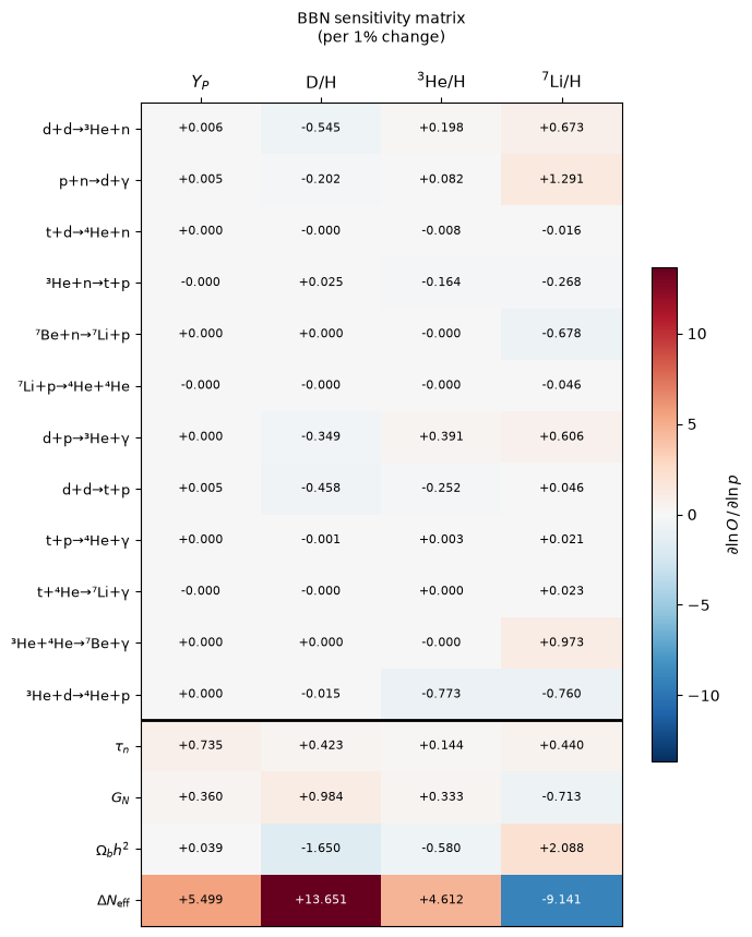
Saved plots/sensitivity_heatmap.pdf
5. Markdown export
to_markdown() produces a table ready to paste into a paper draft, GitHub
issue, or the docs; to_dataframe() returns the same data as a pandas frame.
print(tab.to_markdown())
| Parameter | $Y_P$ | D/H | $^3$He/H | $^7$Li/H |
| --- | --- | --- | --- | --- |
| d+d→³He+n | +0.0061 | -0.5453 | +0.1983 | +0.6734 |
| p+n→d+γ | +0.0045 | -0.2022 | +0.0816 | +1.2911 |
| t+d→⁴He+n | +0.0000 | -0.0002 | -0.0076 | -0.0160 |
| ³He+n→t+p | -0.0000 | +0.0253 | -0.1637 | -0.2682 |
| ⁷Be+n→⁷Li+p | +0.0000 | +0.0000 | -0.0000 | -0.6779 |
| ⁷Li+p→⁴He+⁴He | -0.0000 | -0.0000 | -0.0000 | -0.0458 |
| d+p→³He+γ | +0.0002 | -0.3485 | +0.3910 | +0.6064 |
| d+d→t+p | +0.0052 | -0.4584 | -0.2521 | +0.0456 |
| t+p→⁴He+γ | +0.0000 | -0.0006 | +0.0033 | +0.0207 |
| t+⁴He→⁷Li+γ | -0.0000 | -0.0000 | +0.0000 | +0.0225 |
| ³He+⁴He→⁷Be+γ | +0.0000 | +0.0001 | -0.0000 | +0.9735 |
| ³He+d→⁴He+p | +0.0000 | -0.0146 | -0.7727 | -0.7599 |
| $\tau_n$ | +0.7353 | +0.4230 | +0.1438 | +0.4403 |
| $G_N$ | +0.3596 | +0.9836 | +0.3330 | -0.7127 |
| $\Omega_b h^2$ | +0.0393 | -1.6501 | -0.5799 | +2.0880 |
| $\Delta N_{\rm eff}$ | +5.4993 | +13.6512 | +4.6125 | -9.1411 |